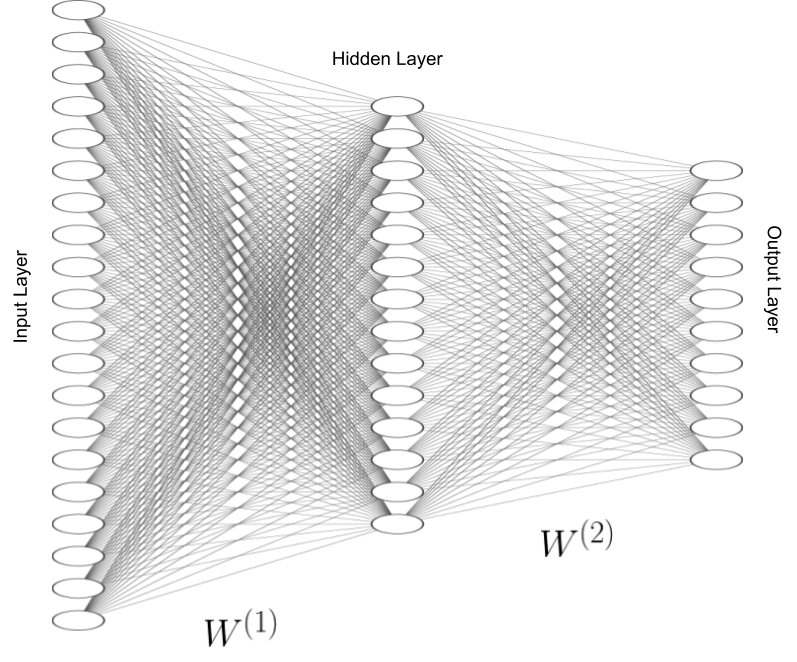
 A fully-connected 2 layer neural network. Made using NN-SVG.
In this assignment we are asked to implement a 2 layer network. To start off lets first draw the 2 layer neural network as a computational graph.
 A circuit diagram representing the 2 layer fully-connected neural network.
The steps in the circuit diagram above represent the forward-pass through the nueral network. It is relative straightforward to implement the forward pass in python:
# Unpack variables from the params dictionary
N, D = X.shape

W1, b1 = self.params['W1'], self.params['b1']
W2, b2 = self.params['W2'], self.params['b2']

# first layer activation
a = np.matmul(X, W1) + b1
a[a<0] = 0
b = a

# second layer activation
scores = np.matmul(b, W2) + b2

#softmax
ytrue_class_prob = np.array([[i, y] for i, y in enumerate(y)])
d = np.exp(scores)
f = d[ytrue_class_prob[:, 0], ytrue_class_prob[:, 1]] / np.sum(d, axis=1).reshape(1, N)

p_ = -np.log(f)
loss = np.sum(p_)
loss /= N
loss += reg * (np.sum(W1 * W1) + np.sum(W2 * W2))
For the backward we first need to calculate the derivative of the loss \(L\) with respect to all elements of the score matrix. The softmax loss of the score matrix is given by
\[\begin{align} L &= \frac{1}{N} \sum_i L_i + \lambda(||W^{(1)}||^2 + W^{(2)}||^2) \nonumber \\ &= \frac{1}{N} \sum_i -\text{log}\frac{e^{score_{i,y_i}}}{\sum_j e^{score_{i,j}}} \nonumber \\ &+ \lambda(||W^{(1)}||^2 + W^{(2)}||^2) \nonumber \\ & = -score_{i,y_i} + \text{log}\sum_j e^{score_{i,j}} + \lambda(||W^{(1)}||^2 + W^{(2)}||^2) \end{align}\]The derivative \(\frac{\partial L}{\partial scores}\) is equivalent to
\[\begin{align} \frac{\partial L}{\partial scores} = \begin{pmatrix} \frac{\partial L}{\partial score_{0,0}} & \frac{\partial L}{\partial score_{0,1}} & \dots \\ \frac{\partial L}{\partial score_{1,0}} & \frac{\partial L}{\partial score_{1,1}} & \dots \\ \vdots & \vdots & \ddots \end{pmatrix} \end{align}\]Lets calculate
\[\begin{align} \frac{\partial L}{\partial score_{i,k}} = \frac{\partial (-score_{i,y_i} + \text{log}\sum_j e^{score_{i,j}})}{\partial score_{i,k}} \end{align}\]where we have ignored the derivative of L2 regularization \(\lambda(||W^{(1)}||^2 + W^{(2)}||^2)\) because it is a constant so its derivative is 0.
If \(k \neq y_i\) then
\[\begin{align} \frac{\partial L}{\partial score_{i,k}} &= \frac{\partial (\text{log}\sum_j e^{score_{i,j}})}{\partial score_{i,k}} \nonumber \\ &= \frac{\partial (\text{log}\sum_j e^{score_{i,j}})}{\partial \sum_j e^{score_{i,j}}} \frac{\partial \sum_j e^{score_{i,j}}}{\partial e^{score_{i,k}} } \nonumber \\ &= \frac{1}{\sum_j e^{score_{i,j}}} e^{score_{i,k}} \end{align}\]We can similarly show that if \(k = y_i\) then
\[\begin{align} \frac{\partial L}{\partial score_{i,y_i}} = -1 + \frac{1}{\sum_j e^{score_{i,j}}} e^{score_{i,y_i}} \end{align}\]Now we can calculate what each element of the matrix \(\frac{\partial L}{\partial scores}\) will be in python:
ytrue_class_prob = np.array([[i, y] for i, y in enumerate(y)])
d = np.exp(scores)
#divide each elemt in the row by the sum of the row
grad_L_wrt_scores = d/np.sum(d, axis=1, keepdims=True)

grad_L_wrt_scores[ytrue_class_prob[:, 0], ytrue_class_prob[:, 1]] -= 1
grad_L_wrt_scores /= N
Now lets go back to the ciruit diagram and use the rules derived in in the lecture 4 handouts to see how \(\frac{\partial L}{\partial scores}\) backpropogates.
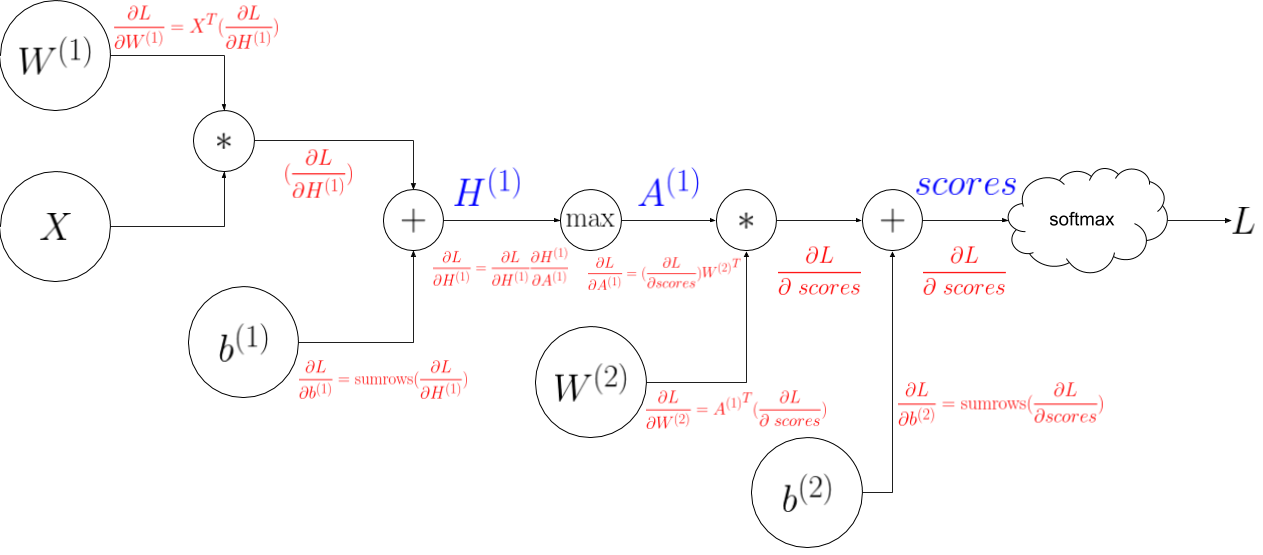 A circuit diagram representing the 2 layer fully-connected neural network. Backprop derivatves are in red.
Here is the python code to implement the backprop shown in the circuit diagram above:
grad_L_wrt_scores = d/np.sum(d, axis=1, keepdims=True)
# print('grad_L_wrt_c: ', grad_L_wrt_c)

grad_L_wrt_scores[ytrue_class_prob[:, 0], ytrue_class_prob[:, 1]] -= 1
grad_L_wrt_scores /= N
# print('grad_L_wrt_c: ', grad_L_wrt_c)
# N * C
grad_L_wrt_W2 = b.T.dot(grad_L_wrt_c)
# print('grad_L_wrt_W2: ', grad_L_wrt_W2)

# N * h
grad_L_wrt_b = grad_L_wrt_c.dot(W2.T)
# print('grad_L_wrt_b: ', grad_L_wrt_b)


grad_L_wrt_b2 = np.sum(grad_L_wrt_c, axis=0)
# print('grad_L_wrt_b2: ', grad_L_wrt_b2.shape)

grad_L_wrt_a = np.where(a <= 0, 0, 1)*grad_L_wrt_b
# print('grad_L_wrt_a: ', grad_L_wrt_a)

grad_L_wrt_W1 = X.T.dot(grad_L_wrt_a)
# print('grad_L_wrt_W1: ', grad_L_wrt_W1)

grad_L_wrt_X = grad_L_wrt_a.dot(W1.T)
# print('grad_L_wrt_X: ', grad_L_wrt_X)

grad_L_wrt_b1 = np.sum(grad_L_wrt_a, axis = 0)
# print('grad_L_wrt_b1: ', grad_L_wrt_b1.shape)

# print('grad_L_wrt_W1.shape: ', grad_L_wrt_W1.shape)
# print('grad_L_wrt_W2.shape: ', grad_L_wrt_W2.shape)


grads['W1'] = grad_L_wrt_W1 + 2 * reg * W1
grads['b1'] = grad_L_wrt_b1
grads['W2'] = grad_L_wrt_W2 + 2 * reg * W2
grads['b2'] = grad_L_wrt_b2
Check out the full assignment here
Comments